Calibrate Sensor Data: Counts to Real Units

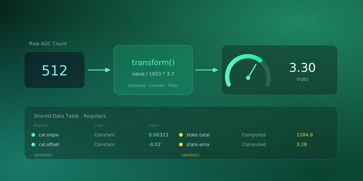
A sensor almost never hands you the number you actually want. A 10-bit ADC gives you 0 to 1023, not volts. A thermistor gives you counts, not degrees. A load cell gives you millivolts, not kilograms. Somewhere between the raw reading and the dashboard, that value has to become a real, calibrated engineering quantity. The interesting question is where that conversion should happen.

Where should sensor calibration happen?

You have three options, and two of them age badly. Convert in firmware, and every recalibration means editing and reflashing the device, a cost that production firmware teams learn to avoid. Convert after the fact in a spreadsheet, and your live dashboard still shows raw counts while you are running the experiment. The middle ground is to convert on the host, live, in a place you can edit without touching the hardware. That is what Serial Studio's dataset transforms are for.

Dataset transforms

Every dataset (each value you plot or display) can carry an optional transform(value) function, written in JavaScript or Lua. The frame parser produces raw values, each raw value is mapped to a dataset, and then, before it reaches the dashboard, the transform converts it. The value it returns replaces the raw one everywhere: widgets, plots, CSV export, MDF4 export, and the API.

Unit conversion is a one-liner:

// Celsius to Fahrenheit
function transform(value) {
  return value * 9 / 5 + 32;
}

Calibrating a raw ADC count to volts has the same shape:

// 10-bit ADC (0..1023) to volts on a 3.3 V reference
function transform(value) {
  return value / 1023 * 3.3;
}

(Both the divide-by-1023 and divide-by-1024 conventions exist; the difference is under a tenth of a percent, so pick one and stay consistent.) If you don't have a sensor wired up yet, the bundled Command-Based ADC Sampling example needs nothing but an Arduino: floating analog pins alone produce a noisy 0-1023 stream you can point this exact transform at.

Transforms are optional, so a dataset without one simply shows the parsed value unchanged. And they fail safe: if the function returns something invalid (undefined, NaN, or it throws), Serial Studio keeps the raw value rather than interrupting the stream.

How do you calibrate a nonlinear sensor, like a thermistor?

A thermistor's resistance does not fall on a straight line with temperature, so a single slope and offset undershoots at one end of its range and overshoots at the other. Serial Studio's transform is a full script, not a fixed formula slot, so the exact nonlinear equation runs in one pass, and a Steinhart-Hart Thermistor template ships in the Transform Editor's built-in list alongside a Polynomial (2nd order) one for other curved responses.

A typical circuit puts the NTC thermistor in a voltage divider with a known fixed resistor. The transform first recovers the thermistor's resistance from the ADC voltage, then solves the Steinhart-Hart equation for temperature, all in the same transform() call:

// NTC thermistor: ADC count -> voltage divider -> Steinhart-Hart -> Celsius
var SERIES_OHMS = 10000;    // fixed resistor in the divider, ohms
var A = 1.009249522e-3;     // Steinhart-Hart constants for this thermistor
var B = 2.378405444e-4;     // (from the datasheet, or fit from 3 known points)
var C = 2.019202697e-7;

function transform(value) {
  var volts = value / 1023 * 3.3;                 // 10-bit ADC, 3.3 V reference
  var resistance = SERIES_OHMS * (3.3 / volts - 1);
  var lnR = Math.log(resistance);
  var kelvin = 1 / (A + B * lnR + C * lnR * lnR * lnR);
  return kelvin - 273.15;                          // Celsius
}

The whole physics chain, voltage-divider algebra plus the cubic log term, is ordinary math running inside one transform() call. Nothing about it is a special case baked into the app; it follows the same one-dataset, one-function contract as the linear example above, just with three constants instead of two.

Most thermistor datasheets list A, B, and C directly for the exact part number. Without one, take three known resistance-and-temperature reference pairs, an ice bath, room temperature, and a calibrated oven work well, and solve the resulting three equations for the constants.

A simpler alternative: two-point calibration

Not every sensor needs three curve-fit constants. When you only have two trustworthy reference points, a two-point calibration draws a straight line between them and reuses the same slope * value + offset shape as the datasheet-based ADC example above:

// Two known references: raw 612 = 0 C (ice water), raw 78 = 100 C (boiling water)
var slope  = (100 - 0) / (78 - 612);
var offset = 0 - slope * 612;

function transform(value) {
  return value * slope + offset;
}

This is the fastest fix when a sensor drifts from unit to unit and the manufacturer's constants aren't handy: measure it at two points you trust, ice water and a rolling boil work for most temperature sensors, and let the two readings define the line. It won't track a curved response as well as Steinhart-Hart does, but the cost is one short calibration session instead of hunting down a datasheet.

xychart-beta
    title "Two-point calibration: line through two trusted references"
    x-axis "Raw ADC count" [612, 478, 345, 212, 78]
    y-axis "Temperature (Celsius)" 0 --> 100
    line [0, 25, 50, 75, 100]

Filtering needs memory

Some conversions have to remember the previous sample. A noisy reading smooths nicely with an exponential moving average, which blends each new value with the last result. Variables declared at the top level of the transform persist between frames, so state is easy to keep:

var alpha = 0.2;
var ema;

function transform(value) {
  ema = (ema === undefined) ? value : alpha * value + (1 - alpha) * ema;
  return ema;
}

Each dataset's top-level state is isolated, so two channels can both run an EMA without clobbering each other's variables. Smoothing like this works in the time domain; when you need to see which frequencies a noisy signal actually contains, the next step is a frequency-domain view of the data.

The magic-number problem, and data tables

Two things get awkward as a project grows, and data tables solve both. First, a calibration constant (a slope, an offset, a full-scale range) often applies to several channels, and copying the number into each transform means you have to edit it in several places later. Second, sometimes one transform computes a value that another needs, like a shared reference or a total across channels.

Serial Studio's answer is data tables: named collections of registers that any transform can read and write. A register has a name, a type, and a value, and it comes in two flavors:

• Constant registers are set when the project loads and are read-only at runtime. Calibration slopes, offsets, and thresholds belong here.
• Computed registers are ordinary memory. A transform writes one with tableSet, and it holds that value until something writes again. This is where running state lives: integrators, counters, filter state, latched flags.

Reading a shared constant keeps the magic number in exactly one place:

function transform(value) {
  const slope  = tableGet("cal", "slope");
  const offset = tableGet("cal", "offset");
  return value * slope + offset;
}

Edit cal.slope once in the Project Editor and every channel that reads it updates together.

A computed register carries a value forward, or hands it to another dataset's transform:

// running total, readable by any other transform
function transform(value) {
  const total = (tableGet("state", "total") || 0) + value;
  tableSet("state", "total", total);
  return total;
}

The full API is small: tableGet and tableSet for the registers, plus datasetGetRaw and datasetGetFinal for reading another dataset's value before or after its own transform has run.

The mental model

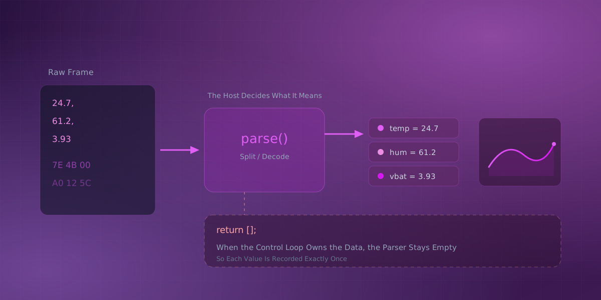
It helps to keep three jobs separate. The frame parser decides what the incoming values are. A transform decides what each value means in real units. Data tables are the shared memory the transforms use to stay consistent and to hold state between frames. Keep those roles distinct and calibration stops being scattered across firmware, scripts, and spreadsheets. And if no built-in widget shows the calibrated result the way you want, you can draw your own.

If the idea of "one owner per value" is new, the companion post How Serial Studio Turns Bytes Into Datasets covers where parsing itself should live. The dataset transforms and data tables references go deeper on both. Once a calibration is dialed in, recording the calibrated session to CSV or MDF4 is what turns it into data you can analyze later instead of just watch live.

Frequently asked questions

Can Serial Studio apply a nonlinear calibration equation directly?

Yes. A transform is a complete JavaScript or Lua function, not a fixed formula slot, so an equation like Steinhart-Hart runs in a single transform() call (Dataset Transforms reference). The Transform Editor even ships a ready-made Steinhart-Hart Thermistor template, alongside a Polynomial (2nd order) one for other curved responses.

What's the difference between a 2-point calibration and a full curve fit?

A two-point calibration draws one straight line through two known references: quick to set up, but only accurate near those two points. A full curve fit like Steinhart-Hart uses three constants to track a sensor's real nonlinear response across its whole range, which matters more the wider that range gets.

Where do the Steinhart-Hart constants (A, B, C) come from?

Most thermistor datasheets list A, B, and C directly for that part number. Without a datasheet, take three known resistance-and-temperature reference pairs and solve the resulting three simultaneous equations for the constants.