Vibration Analysis With a Sound Card and FFT

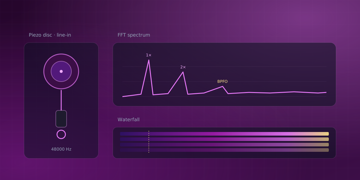
Your computer already contains a two-channel, 16-or-24-bit ADC that samples at 48,000 times per second or better. It is called the sound card, and for questions like "is this motor vibrating more than it did last month," it is a legitimate measurement front end, as a long tradition of sound-card oscilloscope projects attests. Paired with a piezo disc that costs less than a coffee, it will show you a vibration spectrum. This post covers the electronics you need between the disc and the jack, what the spectrum means once you see it, and, just as important, what this rig cannot tell you.

Key takeaways

• A four-part conditioning circuit, bias resistor, series resistor, clamp diodes, DC-blocking capacitor, turns a raw piezo disc into a signal a line-in port can accept safely.
• The sound card's own ADC works as a real spectral instrument once you condition the signal; it's just uncalibrated, good for relative and comparative trending, not absolute severity.
• Machine faults leave known signatures in the FFT: imbalance at 1×, misalignment at 2×, looseness across harmonics, bearing tones at non-integer multiples of shaft speed.
• A waterfall spectrogram turns a run-up or coast-down into a picture, showing exactly where a sliding shaft order crosses a standing resonance.

The sensor and the circuit it needs

A piezo disc is a thin ceramic layer on a brass plate. Strain it and it generates charge; electrically it behaves like a small capacitor in series with a voltage source, which has two consequences. First, it is a very high impedance source. Plugged straight into a typical line input (10 to 47 kΩ), the disc's own capacitance forms a high-pass filter with a corner in the hundreds of hertz, so exactly the low-frequency content you care about gets thrown away. A 1 MΩ load resistor in parallel with the disc moves that corner down to where it belongs. Second, a sharp mechanical impact can generate transients of tens of volts, far beyond the roughly 1 Vrms a consumer line input expects.

So the minimum sensible conditioning is:

1. A 1 MΩ resistor in parallel with the piezo.
2. A series resistor into the port.
3. A pair of back-to-back diodes in parallel with the input to clamp transients.
4. A series capacitor to block DC.

The nicer version adds an op-amp or JFET follower at the sensor so the high-impedance side stays short and the cable is driven at low impedance; the classic sound-card oscilloscope front ends are exactly this circuit. Keep the working signal around half a volt and let the clamp catch the accidents.

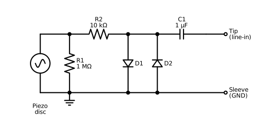
Only R2 and C1 sit in the signal's path; R1 and the diode pair hang in parallel between the signal line and ground. The R2 and C1 values shown are ordinary starting points, not critical choices; anything in the same decade behaves the same way.

What a sound card can and cannot measure

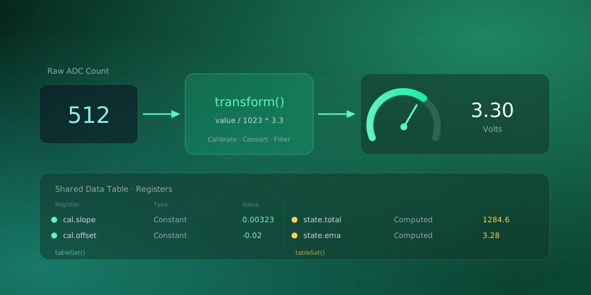
The honest datasheet of this instrument matters more than usual. Line inputs are AC-coupled, so the response rolls off somewhere around 10 to 20 Hz: a shaft turning at 600 RPM has its fundamental at 10 Hz, right at the edge, and anything slower is invisible. On the high end, sample rates of 96 or 192 kHz promise wide bandwidth, but cheap cards keep their anti-aliasing filters tuned for audio, so treat anything above 20 kHz as unverified until you test it. And the amplitude axis is uncalibrated: gain varies by card, by driver, and by the volume slider. Every number you read is in arbitrary units (a dataset transform can rescale them, but it cannot substitute for a calibration). That rules out judging severity against standards like ISO 20816, which is defined in calibrated millimetres per second. What survives is exactly what a prototype bench needs: relative and comparative measurement, on the same rig, over time.

Three traps between the signal and the spectrum

Before reading any spectrum, it is worth knowing the three ways sampled-data analysis can lie to you, because two of them the sound card handles and one it hands to you.

The first is aliasing. The Nyquist-Shannon theorem says a signal sampled at rate fs can only represent frequencies below fs/2; energy above that limit does not disappear, it folds back and reappears at a mirror frequency below, indistinguishable from a real component. The classic victim is the DIY rig: sample a motor with a bare microcontroller ADC at 1 kHz with no filter in front, and a genuine 3.2 kHz bearing tone reappears as a convincing, entirely fictional line at 200 Hz. This is the trap the sound card largely spares you. Audio converters are delta-sigma parts that oversample internally and filter digitally, so within the audio band their anti-aliasing behavior is respectable, which is a real advantage over most cheap acquisition hardware. The residue of the trap moves into the sensor instead: a bare piezo disc has a mechanical resonance of its own, typically a few kilohertz, and a sharp impact makes the disc ring at that frequency like a small bell. A large peak there is often the sensor's own voice, not the machine's.

The second trap is the AC coupling already mentioned, and it deserves its physical statement: a line input contains a series capacitor, so 0 Hz cannot pass, and the response falls away below roughly 10 to 20 Hz. Zero hertz is not an abstraction, it is static displacement and slow drift, and everything slower than the corner is attenuated smoothly rather than cut cleanly, so amplitudes near it are suppressed without warning. This is a hard limit of the instrument, not a setting.

The third trap belongs entirely to you, because it lives in the FFT itself. The transform quietly assumes the captured block of samples is one period of a signal that repeats forever, end spliced to beginning. A tone that completes a whole number of cycles in the block splices perfectly. A tone that does not, which is nearly every real tone, meets its own beginning in a discontinuity, and the energy of that splice smears across the whole spectrum as skirts around the true peak. This is spectral leakage, and untreated it is fatal for machine diagnostics: with no windowing, the skirts of a peak fall off only about 13 dB at the first sidelobe, so the towering 1× peak of ordinary residual imbalance can bury a small bearing tone 30 or 40 dB down, which is precisely the tone you built the rig to find. The cure is a window function, a taper that brings the block's ends smoothly to zero before the transform so the splice vanishes. Hann buys sidelobes about 31 dB down at the cost of a slightly wider peak; Blackman-Harris pushes them below 90 dB for a wider peak still. That trade, sidelobe suppression against frequency resolution, is the whole design space, and for spotting weak tones next to strong ones the suppression wins. Serial Studio's FFT plot applies a Blackman-Harris window for exactly this reason.

xychart-beta
    title "First sidelobe suppression by window"
    x-axis ["No window", "Hann", "Blackman-Harris"]
    y-axis "dB below the main peak" 0 --> 100
    bar [13, 31, 90]

Resolution is the final piece of arithmetic. Bin spacing is fs/N: 48,000 samples per second across a 4,096-point transform gives bins 11.7 Hz apart, fine for separating 1× from a bearing tone on a fast shaft, but too coarse to resolve gear-mesh sidebands spaced at the shaft rate of a slow machine. Finer bins need a longer capture, and a longer capture is a slower-updating waterfall; frequency resolution and time resolution are bought with the same coin.

Reading the spectrum

Machine faults have well-known spectral signatures, all referenced to the shaft's running speed (called 1×).

• Imbalance shows up as a dominant peak at 1×.
• Misalignment tends to raise 2×, and a 2× peak rivaling the 1× is a classic tell.
• Looseness sprays harmonics across the spectrum.
• Bearing defects are the interesting case: rolling-element defect frequencies are non-integer multiples of shaft speed, computable from the bearing geometry (the datasheet-derived BPFO and BPFI figures), so a peak at, say, 3.57× that grows week over week is a bearing race telling you its story.
• Gear mesh adds tooth-mesh frequencies (tooth count times shaft speed) with sidebands spaced at 1×.

A single FFT gives you that snapshot. A waterfall, which stacks spectra over time as a colored map, gives you the dynamics, and it earns its keep during a run-up or coast-down: components tied to shaft speed slide diagonally as the machine accelerates, while structural resonances stand still as vertical ridges. Where a sliding order crosses a standing ridge, the amplitude blooms, and you have found a critical speed without any calibration at all.

Wiring it into a dashboard

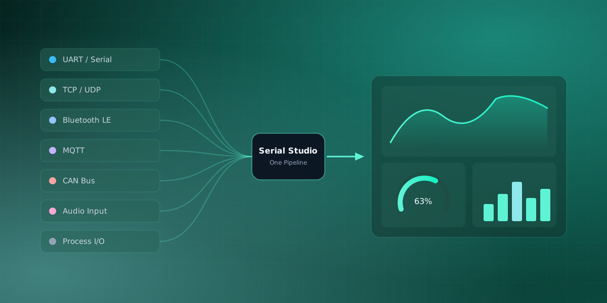
Serial Studio treats audio capture as just another data source, one of several inputs beyond serial ports: the audio input driver (part of Pro) opens the microphone or line-in, and each channel becomes a dataset, one sample per frame, so a 48 kHz capture is a 48,000-frame-per-second stream. In Quick Plot mode the app builds an audio group automatically with the FFT already configured to match the device's sample rate. In a project you assemble it yourself, and there is one setting worth underlining: set the dataset's FFT sampling rate to the actual audio rate, because the default of 100 Hz will scale the frequency axis into nonsense. The FFT plot itself (a free-tier widget, using a Blackman-Harris window) draws the spectrum; the waterfall widget (Pro) draws the spectrogram, reusing the same FFT settings.

From there the workflow is the one described above: mount the disc firmly on the bearing housing (a dab of wax or a magnet base beats tape), capture a baseline spectrum while the machine is known-good, and compare against it later. For before-and-after checks, resonance hunting, and teaching yourself what imbalance looks like, this rig is genuinely good.

Where the cheap rig stops

It is worth saying plainly: this is a qualitative instrument. A real condition-monitoring channel uses an IEPE accelerometer with a calibration certificate stating its sensitivity in millivolts per g, a characterized flat response, and a DAQ with known gain, and that chain is what standards, warranties, and acceptance tests require. The sound-card rig cannot make absolute severity judgments, cannot compare one machine against another, and cannot see slow shafts at all. What it can do is tell you which frequencies are present and whether they are growing, for the price of a piezo disc and an afternoon. For a surprising number of practical questions, that is the whole job.